6 Dynamic models

6.1 Modeling presidential approval with dynamics

At the end of class last week, we knew a couple of things about modeling presidential approval:

presidential approval is stationary, but our measure of consumer sentiment is not. We have to use the first difference if we want to include economic sentiment in a model of approval
if we use OLS to estimate the relative importance of casualties in war, economic sentiment, and the honeymoon period, the residuals are correlated with each other, violating one of the key assumptions behind OLS.

To address the problem of serial correlation, we will use two categories of solutions:

we will incorporate some dynamics in the error term in what is known as an ARIMA model
we will introduce lagged values of the dependent and independent variables in what are known as a dynamic models.

We are going to use two basic approaches to estimate model parameters - the functions in the dyn package and the arima function that is part of base R. For a good, short technical introduction, see Chapter 19, “Time Series Econometrics” in Kennedy (2008)

6.2 The ARIMA model - the special case

The autoregressive integrated moving average (ARIMA) modeling strategy permits us to remedy the problem of serial correlation of the error term. It is then possible to estimate the effect of X on Y in period t. One way to think about this modeling strategy is that all the dynamics - the influence of the past on current observations - is introduced via the error term. This is an assumption implicit in the models we used last week: the effects of X on Y are contemporaneous. There is no way (technically or substantively) in this modeling framework that past values of X cause current values of Y or that past values of Y influence current values of Y - everything about the past comes in via the error term. This already suggests that the ARIMA strategy may be a special case and a more general strategy for handling dynamics may be appropriate.

Maintaining the model specification from earlier examples, the model summarized below treats presidential approval as a function of the first difference in current economic conditions (the Michigan Index of Consumer Sentiment. MICS), total casualties in war during the quarter, and a counter to indicate the honeymoon period (4 in the first quarter of the first year falling to 0 in the first quarter of the second year). (Since I knew the MICS variable was not stationary, I used the first difference in MICS.)

Our remedy relies on some knowledge of the nature of the interdependence of our disturbance terms (\(u\)). Recall, our basic model is:

\[Approval_t = \beta_0 + \beta_1(diff(MICS_t))+ \beta_2(Honeymoon_t) +\beta_3(Casualty_t)+ u_{t}\]

and in order to use the Durbin-Watson test we have assumed that the error is generated by an AR(1) mechanism, where:

\[ –1<\rho< 1 \]

\[ u_t = \rho u_{t-1} + v_t\]

Our goal is to somehow transform our model so that in the transformed model the error term is serially independent (no autocorrelation)

If we can transform the model in that way, then our OLS estimates on the transformed model will be BLUE, assuming all other OLS assumptions are fulfilled. To do that we simply combine the equations above.

\[Approval_t = \beta_0 + \beta_1(diff(MICS_t))+ \beta_2(Honeymoon_t) +\beta_3(Casualty_t)+ \rho u_{t-1} + v_t\]

This transformation can be generalized to higher-order schemes, AR(2), etc., which we will not worry about here. Estimation of this model is simple in R using the arima function.

R implements a nonlinear strategy for simultaneously estimating \(\rho\) and the parameters of the model (\(\beta_i\)). Note that this approach is a contemporary and superior alternative to two techniques that you might see in older journal articles – Prais-Winsten regression and Cochran-Orchutt estimation. Both of these use OLS to get at the same problem. They are two-step approaches - first estimating \(\rho\) and then estimating the parameters given that estimate. These tests typically report the durbin-watson test statistic to evaluate the reduction in serial correlation. If you are reading literature published before, say, 2002, you might see this approach. The substantive and statistical findings should be nearly identical to the ARIMA approach below.

To see the code used to read and transform the data, see working-with-time-series.html#using-the-urca-package-and-the-ur.test-function and working-with-time-series.html#modeling-presidential-approval.

# While I use the dyn package below to estimate
# dynamic models, the arima function requires
# that I create the first difference variable
# and then bind all of the X variables together.

# Create the first difference variable dmics
# this syntax places the first calculated difference in the second row
# if you forget this, you will get an error message
poq$dmics[2:nrow(poq)]<-diff(poq$mics)
xvar<-cbind(poq$dmics, poq$honeymoon, poq$casualty)
# estimate the arima model
arima<-arima(poq$approval, xreg=xvar,  order=c(1,0,0))
# produce the table
stargazer(arima,  type="html",
          model.names=FALSE, model.numbers=FALSE, style="apsr", digits=2,
          dep.var.labels=c("Presidential approval"),
          covariate.labels=c("AR(1)", "Constant", "MICS, first difference",  "Honeymoon", "Casualities"),
          title="**Table 1. Presidential approval as a function of economy, war and the honeymoon. ARIMA**",
          notes= "p<.10* ; p<.05**",  notes.append = FALSE,
          omit.stat=c("ser","f"),
          star.cutoffs = c(0.10,0.05))

**Table 1. Presidential approval as a function of economy, war and the honeymoon. ARIMA**

	Presidential approval

AR(1)	0.88^**
	(0.03)
Constant	53.52^**
	(3.16)
MICS, first difference	0.10^*
	(0.05)
Honeymoon	3.13^**
	(0.43)
Casualities	-0.001
	(0.001)
N	223
Log Likelihood	-700.12
AIC	1,412.23

p<.10* ; p<.05**

There are a couple of things to note about this output.

First, notice we have an estimate for \(\rho\), our ar(1) parameter: 0.88. This indicates a lot of persistence. Closer to 1.0 means that this process - updating approval to new information - takes time - approval is sticky.

Second, I will reproduce basic OLS below, but notice here that the honeymoon variable is significant (+3) and the economic sentiment variable is significant, but not casualties.

We can repeat our test for serial correlation that we employed last week - the B-G test.

# test for serial correlation up to lag 4
# Note that bgtest requires an lm object, so I had to fit a model..
kable(tidy(bgtest(arima$residuals~1, order=4, type = c("Chisq"))), digits=2, caption="**Table 2.  B-G test for serial correlation, ARIMA**")

**Table 2. B-G test for serial correlation, ARIMA**
statistic	p.value	parameter	method
6.06	0.19	4	Breusch-Godfrey test for serial correlation of order up to 4

Finally, notice that the B-G test is insignificant. There is no serial correlation up to lag 4 if we rely on ARIMA.

6.3 Dynamic models using the dyn package (dl, pa, adl, ecm) - a general approach

In order to use the dyn package functions I identify each variable as a time series. Notice that when I then specify the model Is just indicate diff(mics) - the first difference in MICS, rather than using the new variable created above.

We will start with simple OLS and test for serial correlation using the B-G test, the final result from the last chapter.

# Since I only use this library for this chapter, I call it here rather than in _common.R
library(dyn)
# identify each variable as a time series
# this steps give us the ability to use differences and
# lags in the dny models below and to bind the columns for arima
mics<-ts(poq$mics)
approval<-ts(poq$approval)
honeymoon<-ts(poq$honeymoon)
casualty<-ts(poq$casualty)
#DoDspend<-ts(poq$DoDspend)

# estimate the static model with no correction for serial correlation
# approval as a function of the first difference in consumer sentiment, casualties, and the honeymoon period.
# This is where we left off last week.
static<-dyn$lm(approval~diff(mics)+casualty+honeymoon)
# view the model info
stargazer(static,  type="html",
          model.names=FALSE, model.numbers=FALSE, style="apsr", digits=2,
          dep.var.labels=c("Presidential approval"),
          title="**Table 3. Presidential approval as a function of economy, war and the honeymoon. OLS**",
          notes= "p<.10* ; p<.05**",  notes.append = FALSE,
          covariate.labels=c("MICS, first difference", "Casualities", "Honeymoon"), omit.stat=c("ser","f"),
          star.cutoffs = c(0.10,0.05))

**Table 3. Presidential approval as a function of economy, war and the honeymoon. OLS**

	Presidential approval

MICS, first difference	0.14
	(0.16)
Casualities	-0.002^**
	(0.001)
Honeymoon	3.04^**
	(0.74)
Constant	54.58^**
	(0.90)
N	223
R²	0.08
Adjusted R²	0.07

p<.10* ; p<.05**

# generate the residuals and test for serial correlation
kable(tidy(bgtest(static, order=4, type = c("Chisq"))), digits=2, caption="**Table 4.  B-G test for serial correlation, OLS**")

**Table 4. B-G test for serial correlation, OLS**
statistic	p.value	parameter	method
175.62	0	4	Breusch-Godfrey test for serial correlation of order up to 4

Could presidential approval depend on economic conditions in the previous quarter, rather than the current quarter? Isn’t it possible that sentiments may not immediately be updated as objective conditions change? Or, in our case, that those sentiments might not immediately affect our approval of the President? Should we assume this?

Why might lagged effects occur? psychology, intertia, technology, institutions. Think about all that is required for someone to update an attitude or belief. Would it ever be reasonable to think this happens instantly? For a brief discussion of when and why lagged effects might matter, see Section 8.4 “Autocorrelated Disturbances” in Kennedy (2008)

To test for the presence of these longer-term effects, we introduce lagged values of the independent or dependent variables. Models that incorporate lagged variables are dynamic models - since effects of a change in X at time t have effects on later values of Y, at t+1 or t+2.

6.3.1 Distributed lag models

If multiple lagged values of an independent variable are included, then the model is a distributed lag model. The effect of a change in X is distributed over future time periods.

Example: suppose the true model for some outcome was

\[y=1.0+0.6*x_{t-1}+0.4*x_{t-2}+0.2*x_{t-3}\]

If X was stable at 1 for many periods, then Y would be equal to \[1+0.6+0.4+0.2=2.2\]

If X rose to 2 at period t, Y would be equal to:

2.2 at period t (no effect)
2.8 at period t+1
3.2 at period t+2
3.4 at period t+3 (and beyond)

The difference between \(x=1\) and \(x=2\), a one unit change in X, is. in the long-run. the SUM of the coefficients on the lagged value of \(x\): \[0.6+0.4+0.2=1.2\]

The table below reports estimates for an autoregressive distributed lag model that includes 4 lags of the first difference in MICS and 4 lags of the casualty variable.

# estimate the distributed lag model (with four lags of the first difference of mics)
# the stats:: notation indicates I want to use the lag function from the stats package
adl<-dyn$lm(approval~diff(mics)+
           +stats::lag(diff(mics), -1)
           +stats::lag(diff(mics), -2)
           +stats::lag(diff(mics), -3)
           +stats::lag(diff(mics), -4)
           +casualty
           +stats::lag(casualty, -1)
           +stats::lag(casualty, -2)
           +stats::lag(casualty, -3)
           +stats::lag(casualty, -4)
           +honeymoon)

# view the model info
stargazer(adl,  type="html",
          model.names=FALSE, model.numbers=FALSE, style="apsr", digits=2,
          dep.var.labels=c("Presidential approval"),
          title="**Table 5. Presidential approval as a function of economy, war and the honeymoon, ADL(4)**",
          notes= "p<.10* ; p<.05**",  notes.append = FALSE,
          omit.stat=c("ser","f"),
          star.cutoffs = c(0.10,0.05))

**Table 5. Presidential approval as a function of economy, war and the honeymoon, ADL(4)**

	Presidential approval

diff(mics)	0.15
	(0.16)
stats::lag(diff(mics), -1)	0.27^*
	(0.16)
stats::lag(diff(mics), -2)	0.19
	(0.17)
stats::lag(diff(mics), -3)	0.14
	(0.17)
stats::lag(diff(mics), -4)	0.12
	(0.17)
casualty	-0.004
	(0.003)
stats::lag(casualty, -1)	0.002
	(0.004)
stats::lag(casualty, -2)	-0.003
	(0.003)
stats::lag(casualty, -3)	0.002
	(0.003)
stats::lag(casualty, -4)	0.002
	(0.002)
honeymoon	2.55^**
	(0.79)
Constant	54.55^**
	(0.91)
N	219
R²	0.11
Adjusted R²	0.06

p<.10* ; p<.05**

We should treat the coefficient on X_t as the short-run impact.

The sum of the coefficients on the X and its lags is the long-run impact (LRI) or total multiplier. In the example above, the short-run impact of economic sentiment is 0.15 but the long-run multiplier is:

\[0.15+0.27+0.19+0.14+0.12 = 0.87\]

\[LRI=\beta_{X_1}+\beta_{X_1,t-1}+\beta_{X_1,t-2}+...\beta_{X_1,t-n}\]

This means that a 10 unit increase in the MICS would translate - over four quarters - into an 8.7 point increase in presidential approval.

Note one practical problem with this approach. The values of X_t could be highly correlated over time - so the index and the lags are highly correlated with each other. Remember that the effect of collinearity is to increase standard errors. Since we are using first differences for economic sentiment in this model, this is not a problem, but in can be problem in many applications, including our use of the raw series for casualties.

We don’t have any correction for serial correlation here and the white noise test indicates that the serial correlation is still a problem even after we introduced the lagged values of X.

# generate the residuals and test for serial correlation
kable(tidy(bgtest(adl, order=4, type = c("Chisq"))), digits=2, caption="**Table 6.  B-G test for serial correlation, ADL(4)**")

**Table 6. B-G test for serial correlation, ADL(4)**
statistic	p.value	parameter	method
170.19	0	4	Breusch-Godfrey test for serial correlation of order up to 4

6.3.2 Partial adjustment models (lagged value of approval)

If the lagged value of the dependent variable is included, then the model is a partial adjustment model. This model specification is designed to overcome the potential problem of collinearity in the distributed lag model. Using this model specification, the OLS estimator only performs well in large samples and in the absence of serial correlation - the data and the residuals must be stationary.

You will see this in practice when we talk about working-with-time-series-cross-sectional-tscs-data.html#replicating-democratization-and-international-border-settlements. It is the strategy used for a panel model testing the link between settled borders and the polity2 score in Owsiak (2013).)

For the approval data, the basic model is estimated via OLS:

\[approval_t=\beta_0+\beta_1diff(mics)_t+\beta_2casualty_t+\beta_3honeymoon_t+ \beta_4approval_{t-1}\]

pa<-dyn$lm(approval~diff(mics)
             +casualty
             +honeymoon
             +stats::lag(approval, -1))

# view the model info
#stargazer (pa, style="qje", type="text" , omit="factor" , dep.var.labels = c("Presidential approval", "\n"), digits=2, title=c("Partial adjustment model"), omit.stat=c("ser","f"),column.sep.width=c("12pt"))
# produce the table
stargazer(pa,  type="html",
          model.names=FALSE, model.numbers=FALSE, style="apsr", digits=2,
          dep.var.labels=c("Presidential approval"),
          covariate.labels=c("MICS, first difference", "Casualities", "Honeymoon", "Approval, first lag", "Constant"),
          title="**Table 7. Presidential approval as a function of economy, war and the honeymoon, Partial Adjustment**",
          notes= "p<.10* ; p<.05**",  notes.append = FALSE,
          omit.stat=c("ser","f"),
          star.cutoffs = c(0.10,0.05))

**Table 7. Presidential approval as a function of economy, war and the honeymoon, Partial Adjustment**

	Presidential approval

MICS, first difference	0.33^**
	(0.08)
Casualities	-0.0002
	(0.0005)
Honeymoon	2.69^**
	(0.37)
Approval, first lag	0.84^**
	(0.03)
Constant	7.46^**
	(1.86)
N	223
R²	0.78
Adjusted R²	0.77

p<.10* ; p<.05**

# generate the residuals and test for serial correlation
kable(tidy(bgtest(pa, order=4, type = c("Chisq"))), digits=2, caption="**Table 8.  B-G test for serial correlation, PA**")

(#tab:bg_test5)**Table 8. B-G test for serial correlation, PA**
statistic	p.value	parameter	method
7.4	0.12	4	Breusch-Godfrey test for serial correlation of order up to 4

A couple of features of the output are noticeable - now we are introducing persistence in the outcome directly in the model. About 84% (0.84) of last quarter’s approval rating carries over. And the effect of consumer sentiment is large when you use this strategy.

The coefficient on X can be interpreted as the short-run impact. The long run impact is calculated as \(\beta_1 / (1-\beta_4)\).

\[LRI=\beta_{X1} / (1.0-\beta_{Y,t-1})\]

These results suggest that the short-run impact is 0.33 and the long-run impact is: \[0.33/(1-0.840)=2.061\]

A 10 point jump in the Michigan Index of Consumer Sentiment will translate into a 20.6 point increase in presidential approval, all other things equal, in the long run.

Note the slight difference between the two modeling approaches – in the ADL. the long run effect is about six times larger than the short-run effect. In the PA model, the long run effect is about seven times larger. This is due to the fact that the long run effect plays out over larger number of lags. .33 at t, .33.88 at t+1, ,33.84*.84 at t+2….

Autoregressive distributed lag (lagged value of approval and first lag of difference in MICS)

In an autoregressive distributed lag model, lagged values of both the independent variable and the dependent variable are included. The most common form of this model is the ADL (1,1) model:

\[Y_t=\beta_0+\beta_1X1_t+\beta_2X1_{t-1} +\beta_3X2_t+\beta_4X2_{t-1}+\beta_5Y_{t-1}\] Note how general this model is. If \(\beta_2=0\) and \(\beta_4=0\) then we have a partial adjustment model. If \(\beta_5=0\). then we have a distributed lag model.

In the long-run, the effect of a one unit change in X1 would be calculated:

\[LRI=(\beta_{X1,t}+\beta_{X1,t-1)}/(1-\beta_{Y,t-1})\]

# estimate the distributed lag model (with one lag of the first difference of mics and casualties)
padl<-dyn$lm(approval~diff(mics)+
           +stats::lag(diff(mics), -1)
           +casualty
           +stats::lag(casualty, -1)
           +honeymoon
           +stats::lag(approval, -1))

# produce the table
stargazer(padl,  type="html",
          model.names=FALSE, model.numbers=FALSE, style="apsr", digits=2,
          dep.var.labels=c("Presidential approval"),
          title="**Table 9. Presidential approval as a function of economy, war and the honeymoon, PADL**",
          notes= "p<.10* ; p<.05**",  notes.append = FALSE,
          omit.stat=c("ser","f"),
          star.cutoffs = c(0.10,0.05))

**Table 9. Presidential approval as a function of economy, war and the honeymoon, PADL**

	Presidential approval

diff(mics)	0.32^**
	(0.08)
stats::lag(diff(mics), -1)	0.17^**
	(0.08)
casualty	-0.0005
	(0.001)
stats::lag(casualty, -1)	0.0003
	(0.001)
honeymoon	2.36^**
	(0.36)
stats::lag(approval, -1)	0.86^**
	(0.03)
Constant	6.77^**
	(1.79)
N	222
R²	0.80
Adjusted R²	0.79

p<.10* ; p<.05**

The coefficient on X can be interpreted as the short-run impact. The long run impact is calculated as

\[LRI_{mics}=(\beta_{d.mics}+\beta_{lag(d.mics)}) / \beta_{Y_{t-1}} \]

These results suggest that the short-run impact is 0.32 and the total long-run impact is \((0.32+0.17)/(1.0-0.86)=3.1\). Most of the effect is after the first period.

In this case, the test for serial correlation indicates that there is no longer any serial correlation in the residuals.

# generate the residuals and test for serial correlation
kable(tidy(bgtest(padl, order=4, type = c("Chisq"))), digits=2, caption="**Table 10.  B-G test for serial correlation. PADL**")

(#tab:bg_test6)**Table 10. B-G test for serial correlation. PADL**
statistic	p.value	parameter	method
5.72	0.22	4	Breusch-Godfrey test for serial correlation of order up to 4

6.3.3 Error Correction Models

A variant of the model above is becoming more widely used in political science. Some recent work (mainly by Suzanne DeBoef [Linn]) focuses on the long run relationship between two times series, series that may in fact share a trend (both nonstationary!). The solution is called an error correction model (ECM). The logic of the error correction model is that there is a long run relationship between two series and it takes many periods for changes in X and Y to be incorporated. For this set of models, we will use the nonstationary raw MICS series.

Initial versions of the ECM used a two-step process. Simple OLS was applied to the relationship between X and Y. We observe if the relationship is statistically significant and if the residuals have no unit root - if so this is known as a cointegrating regression. We then include the lag of the residual in a regression of the difference in Y on the lag of X. But, since we know that the first stage may be biased and inefficient if X or Y contain unit roots, we estimate the parameters of both models jointly. The algebra for this transformation is outlined in De Boef and Keele (2008). The general form of the model, known as the single equation error correction model becomes:

\[Y_t-Y_{t-1}=\beta_0 + \beta_1Y_{t-1}+\beta_2 X_{t-1}+ \beta_3(X_t-X_{t-1})+e_t\]

In this case, \(\beta_2\) is the short-run effect and the long run effect is:

\[LRI=\beta_3 / -\beta_1\]

This approach has the considerable advantage that it can be applied to both stationary and nonstationary (unit root) processes. We overcome the serial correlation problem by directly modeling the dynamics in the model, not the error term. We overcome the nonstationary problem by getting the stationary error term worked into the model. There is also a compelling behavioral story too - current period differences in Y are a function of the short-term impact of X and the extent to which Y was out of equilibrium with respect to X in the previous period. You could have a very nuanced empirical story explained and incorporated in this model - involving a mixture of short-term and long-term effects. Technically the model is uncomplicated.


ecm<-dyn$lm(diff(approval)~
            +stats::lag(approval, -1)
            +stats::lag(mics, -1)
            +diff(mics)
            +stats::lag(casualty,-1)
            +diff(casualty)
            +stats::lag(honeymoon,-1)
            +diff(honeymoon))


# view the model info
# produce the table
stargazer(ecm,  type="html",
          model.names=FALSE, model.numbers=FALSE, style="apsr", digits=2,
          dep.var.labels=c("Presidential approval"),
          title="**Table 7. Presidential approval as a function of economy, war and the honeymoon, ECM**",
          notes= "p<.10* ; p<.05**",  notes.append = FALSE,
          omit.stat=c("ser","f"),
          star.cutoffs = c(0.10,0.05), column.sep.width=c("12pt"))

**Table 7. Presidential approval as a function of economy, war and the honeymoon, ECM**

	Presidential approval

stats::lag(approval, -1)	-0.17^**
	(0.04)
stats::lag(mics, -1)	0.13^**
	(0.04)
diff(mics)	0.37^**
	(0.08)
stats::lag(casualty, -1)	-0.0002
	(0.0005)
diff(casualty)	-0.002
	(0.001)
stats::lag(honeymoon, -1)	2.01^**
	(0.39)
diff(honeymoon)	3.99^**
	(0.43)
Constant	-2.62
	(3.00)
N	223
R²	0.40
Adjusted R²	0.39

p<.10* ; p<.05**



# generate the residuals and test for serial correlation
bgtest(ecm, order=4, type = c("Chisq"))

Breusch-Godfrey test for serial correlation of order up to 4

data: ecm LM test = 7.1651, df = 4, p-value = 0.1274 Thes short run effect is 0.13, but the long run effect estimated with ECM is:

\[(0.37)/(-(-0.17))=2.17\]

A 10 point increase in the MICS would generate a 21.7 point increases in approval.

The ECM and DL(1) models are very similar except – and this is where the ECM has an advantage – the left hand side dependent variable is a first difference. To see these similarities, both models are side-by-side, below.

To simplify the table, I just use MICS and defense spending as predictors. Notice that this is the level of MICS, not the difference as our X variable.


ecmx<-dyn$lm(diff(approval)~
            stats::lag(approval, -1)
            +stats::lag(mics, -1)
            +diff(mics)

            )

adl1x<-dyn$lm(approval~
           stats::lag(approval, -1)
           +mics
           +stats::lag(mics, -1)

            )


# view the model info
# produce the table
stargazer(ecmx, adl1x,  type="html",
          model.names=FALSE, model.numbers=FALSE, style="apsr", digits=2,
          dep.var.labels=c("Presidential approval"),
          title="**Table 8. Presidential approval as a function of economy, war and the honeymoon, SSDPADL**",
          notes= "p<.10* ; p<.05**",  notes.append = FALSE,
          omit.stat=c("ser","f"),
          star.cutoffs = c(0.10,0.05))

**Table 8. Presidential approval as a function of economy, war and the honeymoon, SSDPADL**

	Presidential approval	approval ~ stats::lag(approval, -1) + mics + stats::lag(mics, -1)

stats::lag(approval, -1)	-0.20^**	0.80^**
	(0.04)	(0.04)
mics		0.35^**
		(0.09)
stats::lag(mics, -1)	0.13^**	-0.21^**
	(0.04)	(0.09)
diff(mics)	0.35^**
	(0.09)
Constant	-0.50	-0.50
	(3.49)	(3.49)
N	223	223
R²	0.16	0.73
Adjusted R²	0.15	0.73

p<.10* ; p<.05**


# generate the residuals and test for serial correlation
bgtest(ecmx, order=4, type = c("Chisq"))

Breusch-Godfrey test for serial correlation of order up to 4

data: ecmx LM test = 6.9034, df = 4, p-value = 0.1411

bgtest(adl1x, order=4, type = c("Chisq"))

Breusch-Godfrey test for serial correlation of order up to 4

data: adl1x LM test = 6.9034, df = 4, p-value = 0.1411

In the table above, the long-run effect of the MICS in the ADL model is:

\[(0.347+-0.212)/(1-.0796)\]

which is identical to the long-run effect in the ECM model, which is:

\[0.134/(-(-0.204))\]

6.4 A couple of notes about other models

6.4.1 A state-specific dynamic model

We can also deploy interaction terms.

ssd<-dyn$lm(approval~diff(mics)+
            +stats::lag(approval, -1)
            +diff(mics):stats::lag(approval, -1)
            +casualty
            +honeymoon )

# view the model info
# produce the table
stargazer(padl,  type="html",
          model.names=FALSE, model.numbers=FALSE, style="apsr", digits=2,
          dep.var.labels=c("Presidential approval"),
          title="**Table 11. Presidential approval as a function of economy, war and the honeymoon, SSDM**",
          notes= "p<.10* ; p<.05**",  notes.append = FALSE,
          omit.stat=c("ser","f"),
          star.cutoffs = c(0.10,0.05), column.sep.width=c("12pt"))

**Table 11. Presidential approval as a function of economy, war and the honeymoon, SSDM**

	Presidential approval

diff(mics)	0.32^**
	(0.08)
stats::lag(diff(mics), -1)	0.17^**
	(0.08)
casualty	-0.0005
	(0.001)
stats::lag(casualty, -1)	0.0003
	(0.001)
honeymoon	2.36^**
	(0.36)
stats::lag(approval, -1)	0.86^**
	(0.03)
Constant	6.77^**
	(1.79)
N	222
R²	0.80
Adjusted R²	0.79

p<.10* ; p<.05**



# generate the residuals and test for serial correlation
bgtest(ssd, order=4, type = c("Chisq"))

Breusch-Godfrey test for serial correlation of order up to 4

data: ssd LM test = 7.2099, df = 4, p-value = 0.1252

6.4.1.1 Graphing conditional marginal effects (without using cplot).

# Adapted from
## Two-variable interaction plots in R
## Anton Strezhnev 
## 06/17/2013

# Extract Variance Covariance matrix
  covMat = vcov(ssd)
# Get coefficients of variables
  beta_1 = ssd$coefficients["diff(mics)"]
  beta_3 = ssd$coefficients["diff(mics):stats::lag(approval, -1)"]
# Create list of moderator values at which marginal effect is evaluated
  x_2 <- seq(from=5, to=95, by=5)
  # Compute marginal effects
  delta_1 = beta_1 + beta_3*x_2
# Compute variances
  var_1 = covMat[2,2] + (x_2^2)*covMat[6,6] + 2*x_2*covMat[2,6]
# Standard errors
  se_1 = sqrt(var_1)
# Upper and lower confidence bounds
  z_score = qnorm(1 - ((1 - 0.95)/2))
  upper_bound = delta_1 + z_score*se_1
  lower_bound = delta_1 - z_score*se_1
figure_data<-as.data.frame(cbind(x_2,delta_1,upper_bound, lower_bound))

# Figure 2
ggplot(figure_data, aes(x = x_2, y = delta_1)) +
  geom_line(lwd = 1.5) +
  geom_line(aes(y = upper_bound)) +
  geom_line(aes(y = lower_bound)) +
  ggtitle("Figure 2. Marginal effect of economic sentiment, by level of approval") +
   theme(plot.title.position = "plot", plot.title = element_text(face="bold")) +
  labs(x="Approval", y="Marginal effect of first difference in MICS")+
  geom_hline(yintercept=0.00, lty=2)+
  geom_vline(xintercept=mean(poq$approval, na.rm=TRUE), color="red", lty=2)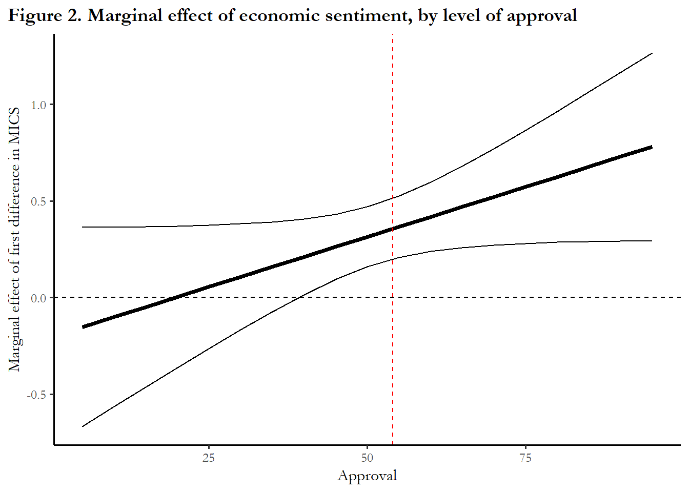

The figure suggests that improving economic sentiment can impact and increase presidential approval when approval is above average or high, but there is no effect (0.0) on approval when approval is low (at or below 40). This describes the experience of President Trump and the persistence of low approval ratings in the face of good economic performance.

6.4.2 Vector AutoRegression or VAR

Some time series analysts bridle at the restrictive nature of the family of models above – why don’t we let the impact of the lagged variables take a more general form – where perhaps the size and direction of the lagged effects varies in some way other than a simple distributed lag. In economics, the classic article is Sims (1980).

And why assume to X->Y – couldn’t it be the case that Y->X in many applications? These objections led to a modeling strategy labeled Vector Autogression or VAR.

In this framework, theory dictates what variables are included in the model, but there is no theory that informs inclusion or exclusion of particular lag or the direction of causal effects. The modeling strategy is parameter- intensive – a lot of parameters are estimated from a modest amount of data. In fact, the number of estimated parameters is so large that often results are summarized in figures – known as impulse response functions.

We won’t cover these models but you can recognize them in practice with the characteristic figures, rather than tables of coefficients. Just recognize that they are dynamic models, estimated with time series, with or no restriction imposed by theory.

5 Working with time series

7 Working with panel data