4 Measures of association: t-test
4.1 What is the t-test?
In many research situations, the \(Y\) variable is some type of scale - either an interval or an ordinal variable. This would include concrete measures like household income, year of education, or age and concepts that we order in a meaningful way – like ideology (from extreme liberal to extreme conservative) or party identification (from strong Democrat to strong Republican) or a feeling thermometer (from 0 – don’t like it – to 100- really like it). But the \(X\) variable may be a category: race, marital status, gender, employment status. If you are interested in determining the relationship between two variables when \(Y\) is a scale, and \(X\) is a category, then a t-test is the appropriate measure of association.
We have used statistics (mean, median, and standard deviation) to describe individual variables. We will use a simple test statistic (t-test) to determine if two groups in a sample are different. T-tests are most appropriate and informative when you compare two groups (male/female, working / not working, Northern/Southern) on a continuous scale.
Recall that we use measures of association to describing relationships between variables. We identify a dependent variable (\(Y\)), an independent variable (\(X\)), and we have a theory about how \(X\) influences \(Y\). The measure of association helps use be precise and clear about three things: - the direction of relationship (does changing from one category of \(X\) to another increase (+) \(Y\) or decrease (-) \(Y\) - the size of the effect (does \(X\) have a big impact on \(Y\) or small?) - whether or not effects in the sample are statistically significant (Could the observed effect be due to chance or sampling error)?
We covered size and direction in Chapter 3, so the focus of this chapter is broadening your understanding of statistical significance. To do this, we talk about inference and introduce the concept of a sampling distribution. After the preliminaries, we review some t-test output related to the National Rifle Association (NRA) feeling thermometer. At the end of the chapter, you should have a sense of what statistical significance means.
4.2 What is inference? And what does this have to do with random samples?
Inference is learning about something we cannot observe from something we can observe. We can observe samples. We cannot observe and measure populations. Inference is learning about populations from samples. In order to make an unbiased inference about a population from a small sample, the only requirement is the sample is random. Any individual in the population has an equal chance of showing up in the sample.
Polling organizations devote a lot of time and energy to figure out how to create random samples. Today, pollsters may rely on face-to-face, phone or web-based contacts to collect data – each strategy has its challenges and face-to-face is obviously very costly. All of these strategies introduce what is known as survey response bias or non-response bias – individuals who are willing to respond may be different than individuals not willing to respond. Before caller id and cell phones, a pollster could randomly dial phone numbers and, as long as the people who answered were willing to talk, the sample would be random. Today, people who are not interested in politics may be the ones who never answer an unidentified caller and cell phone users may not answer at all. There are technical fixes for all of this, but it remains a continuing challenge to make sure a sample is random.
Even if we do have a random sample we know we will be uncertain about how close our sample resembles the larger population – we know that, even if the sample is completely random, we can never have a perfect representation of the population there will be what is known as sampling error. We could get a sample that, by chance, has a lot of Republicans – that would give us a flawed estimate of the average party identification.
We use random sampling since we want to make inferences about the population from our sample. If the samples are random, then descriptive statistics – measures of dispersion or central tendency – also have sampling distributions with known properties. This turns out to be a crucial insight that underpins the way we use statistics to improve what we can say we know from a sample. We explore the sampling distribution of the mean so you can see exactly how this works.
4.3 Sampling distribution of the mean
The mean has a sampling distribution – we didn’t talk about this in Chapter 2 since I wanted to focus on interpretation of descriptive statistics rather than the sampling distributions.
Consider an experiment: If we took 1,000 random samples (or any really large number of samples) from a population it happens to be the case that the sample means – the means from each of the 1,000 samples - are distributed normally with some features we understand,
The mean of the sample means is equal to the population mean (the sample mean is an unbiased estimate of the population mean). On average, our random samples will be accurate.
The standard deviation of the sampling distribution will be equal to the standard deviation of the variable in the population (approximated with standard deviation of the sample) divided by the square root of the sample size. Formally:
\[ \sigma_{M} = \frac{\sigma}{\sqrt{n}} \]
As the sample size gets larger, the width of the sampling distribution gets smaller. If your sample starts to approach the population size, you can imagine no sample would be very different from the population. With very small samples, you could get means very different from the true population mean.
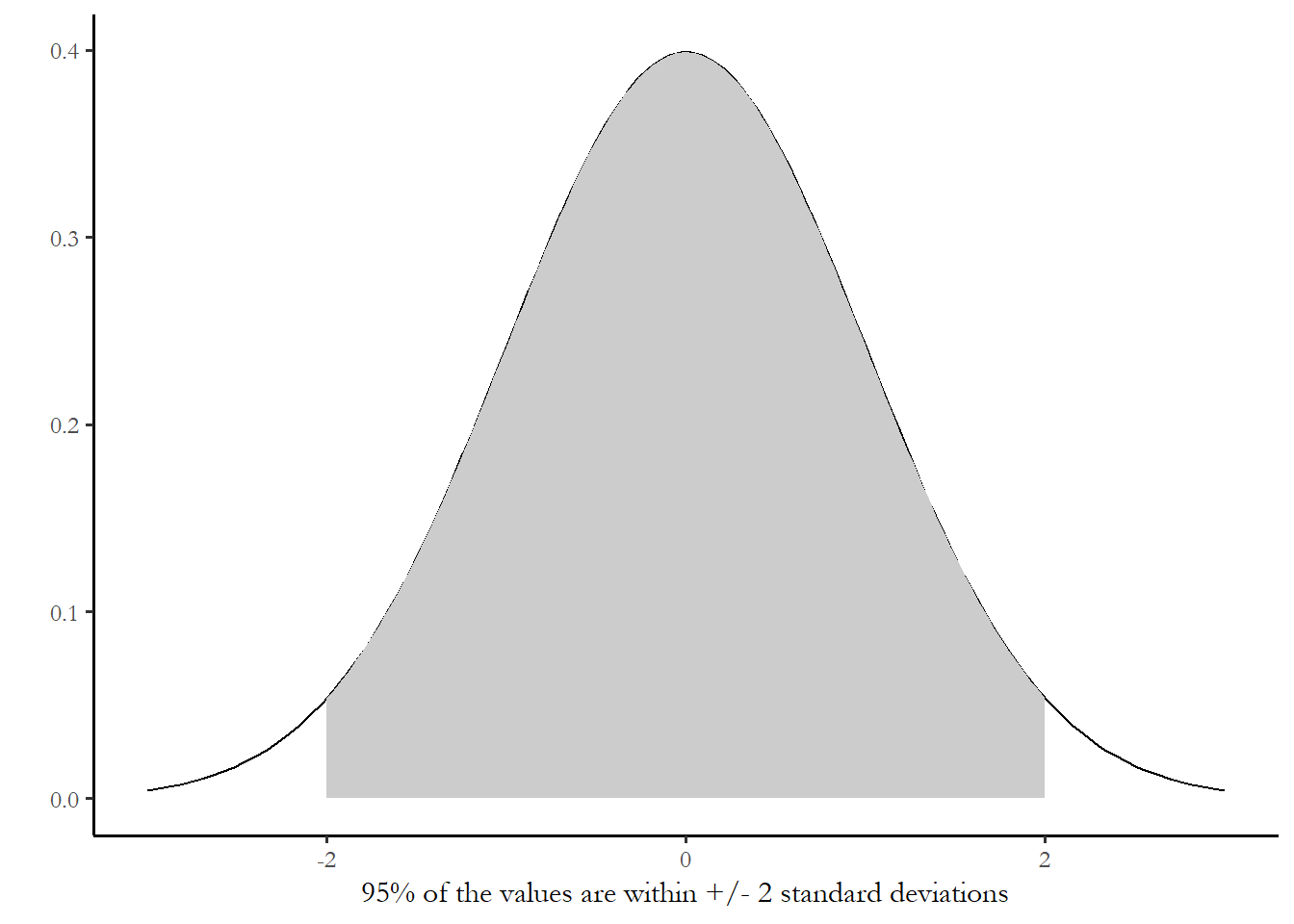
Since we know the mean and standard deviation of this normal distribution, we can exploit other things we know about the normal distribution. Figure 4.1 shows a standard normal distribution - a distribution with a mean of zero and a standard deviation of one. We know – from statistics that 95% of the area covered by this distribution if between -2 and +2 standard deviations from the mean.
So, since our sampling distribution is also normal, we know that any 95% of the samples we draw in our experiment would be within -2/+2 standard deviations of the mean. This is a powerful fact we will leverage to make an inference about the population from our sample.
Figure 4.1 The standard normal distribution
Calculating the margin of error
We know that 95% of the reported values from a large number of repeated samples will be within approximately 2.0 standard deviations (technically, 1.96) of the population mean. The margin of error associated with any random sample is:
\[ME=2*\sigma_{M}=2*\frac{\sigma}{\sqrt{n}}\] If you have in front of you data from a single random sample – you can use software to compute the mean and standard deviation, and knowing the sample size, you can report an estimate for the population mean +/- the margin of error. Table 4.1 reports the descriptive statistics for age in the 2020 ANES. The average respondent in the sample is 47.3 years old. What does that tell us about the population?
Table 4.1 Descriptive statistics for age in the 2024 ANES
| Descriptive statistics | |
|---|---|
| N | 2759 |
| Mean | 48.06 |
| Median | 48 |
| Variance | 326.66 |
| Standard deviation | 18.07 |
Using the formula above, the standard error of the mean would be:
\[ \sigma_M=18.07 / \sqrt{2759} = 0.344 \] \[ ME = 2 * 0.344=0.688\] We know (with 95% certainty) that the population mean is +/- 2 standard error of the means from the sample mean. The 95% confidence interval is 48.06 +/- 0.688 years. That is remarkable – we can be very confident that we know the true age of the actual very large US electorate within less than about 9 months (0.75 of a year).
The key lesson: the “margin of error” associated with the survey response is 2 times the standard error of the mean.
Margin of error and sample size
For a question that has a Yes/No (1/0) answer, the standard deviation cannot be more than about 0.5 for large samples. The highest standard deviation would be a 50% yes and 50% no response or mean 0.5. Half of the responses (“1”s) would be 0.5 above the mean. Half of the responses would be 0.5 below the mean. So the calculation for the standard deviation would be about 0.5 for as n/n-1 gets close to 1 (large samples)
So for a sample of 1000 voters the standard error of the mean would be:
\[\sigma_M = 0.5/ \sqrt{n} = 0.50 / \sqrt{1000} = 0.16\] So we could be confident that our population mean would be within +/- 2 x the standard error = 0.032 or 3.2% of the sample mean of 50%.
As you see on the news, if you ask 1,000 people if they favor or do not favor a particular proposal, the margin of error is roughly +/- 3%
One implication to note here. What if we were to consider how the collection of additional information would improve our estimates? Since the standard error of the mean drops as the sample size gets larger (we are dividing by the square root of the number of observations), each new observation improves our estimates. The figure below shows this improvement for the 0/1 question example above. Assuming the standard deviation is 0.5, we can see how the margin of error declines as the sample size increases.
Figure 4.2 Margin of error if sample standard deviation ~ 0.5, for samples from 100 to 2500
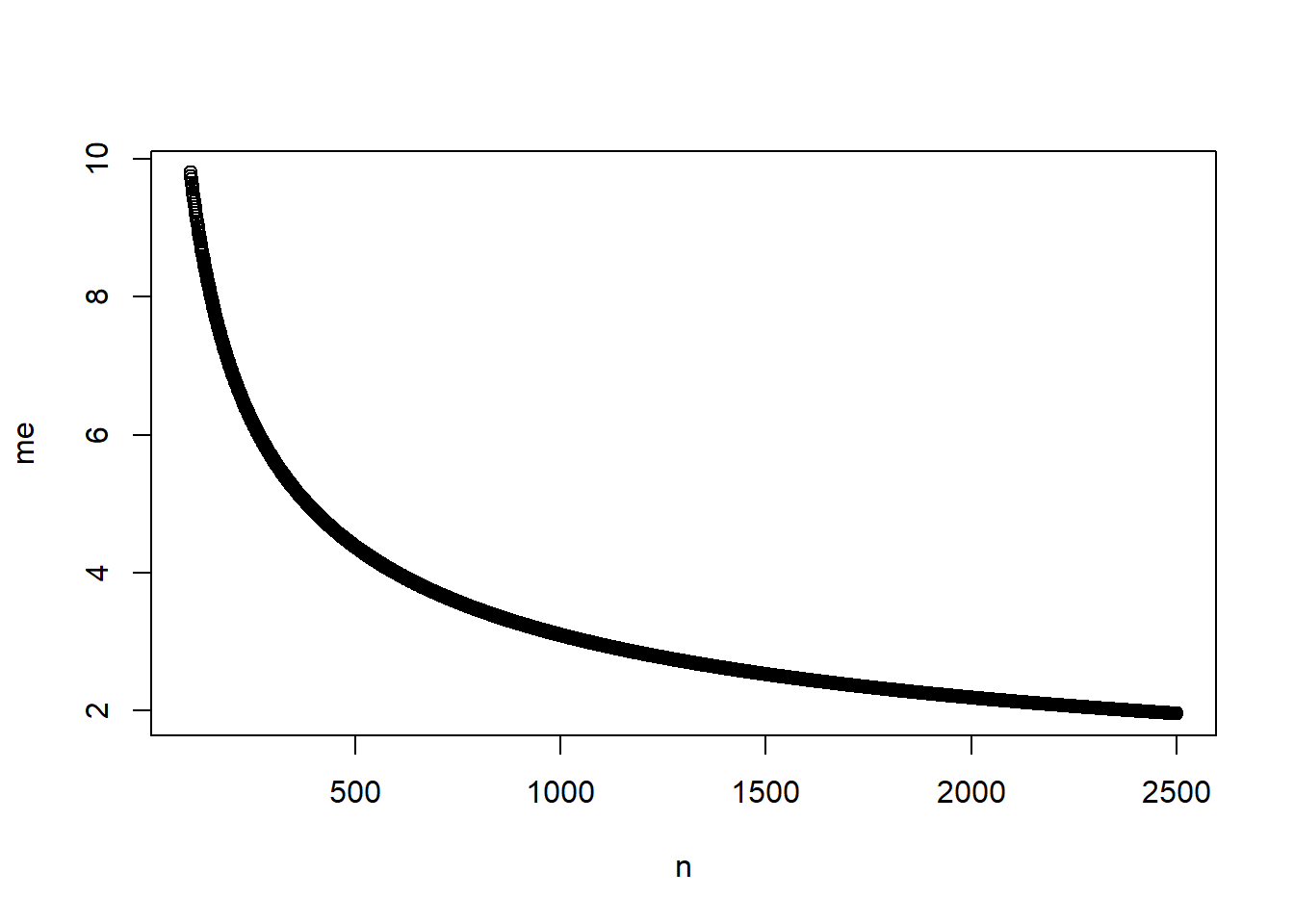
You can see that there is an obvious and large gain in improvement as you move from 500 to 1,000 observations, but much smaller as you move from 1,000 to 1,500. You may see much larger samples in practice - for two reasons. First, some times we need very precise estimates - you wouldn’t, for instance, want to estimate the unemployment rate at +/- 2 percent - economic policy choices require a more much precision. Second, you might be interested in subsets of the population. If you want a decent margin of error associated with attitudes or behavior of minorities, then you would need a very large overall sample, so that the minority sample of interest was closer to 1,500.
4.4 T-test: comparing means for two groups
If we have a sample mean for some variable for some group, we can use that information along with the number in each group and the standard deviation of the responses in each group to make an inference about the mean for that group in the population. We could estimate the average age of women, for instance. A t-test extends this idea to compare samples of two groups – the idea is that we treat our two groups as two independent samples from the same population. If they are in fact identical then they should have the same sample mean. If the sample means are different, then maybe the two groups are different in the population.
The two-sample t-test permits you to test the difference in means across two categories of respondents (2 samples). The output reveals the direction, size, and significance of the effect – Group 1 has a higher or lower mean than Group 2, the difference between the two means is large or small, and the difference between the two means is statistically significant or not.
The sampling distribution of the differences in two means has the t-distribution. We use the t-distribution to evaluate our observed t to determine if observed differences are statistically significant,
The computation is not difficult. Recall that \(\mu\) designates the mean, \(\sigma\) designates the standard deviation, and \(n\) designates sample size. If you have simple descriptive statistics for two samples, you could easily calculate this by hand. Note that \(\mu_1\) designates the mean for group 1 and \(\mu_2\) designates the mean for group 2.
\[t=\frac{(\mu_1-\mu_2)} {\sqrt{(\sigma_1^2/n_1)+(\sigma_2^2/n_2)}}\]
Note: if the sample means are identical, the value of t is zero. As the sample means diverge, the value of t will increase.
The t distribution
Why the “t” distribution? The difference between two means is normally distributed for large samples. The t-distribution approximates this normal distribution in large samples. For small samples, the distribution of differences in the mean is not quite normal. This discrepancy was noted by an experimental brewer at Guinness (W.S. Gossett). Since quality control could involve only small samples of ingredients (malt, hops), the statisticians required a test statistic that performed well for small samples. The t-distribution was widely used after this insight. Gossett and Pearson (the statistician most closely associated with correlation) worked together for a short time at and published their findings in 1896 (correlation/Pearson), 1900 (chi-square/Pearson) and 1908 (t-distribution/Gossett). For details see Porter (1986) or Ziliak (2008).
Later work – attributed to Fisher – resulted in the rule-of-thumb: if a t test value is larger than +2 or smaller than -2, the observed difference in means is statistically significant (more on this below!).
4.5 An application: feelings toward the National Rifle Association
The 2024 ANES includes a number of variables that are all feeling thermometers. A “0” indicates that you do not like the group, person or symbol that the thermometer refers to. A “100” indicates you very much like that group, symbol or person.
There is a feeling thermometer for the NRA. Other group thermometers include the CDC, unions, the military, and big business. Figure 4.3 summarizes the distribution of the NRA thermometer. You can see that most people are neutral, but there are a substantial number who have negative feelings (0) and a large number with positive feelings (75 and 100). Table 4.3 reports the descriptive statistics for the NRA feeling thermometer for the entire sample.
Figure 4.3 Feelings toward the NRA
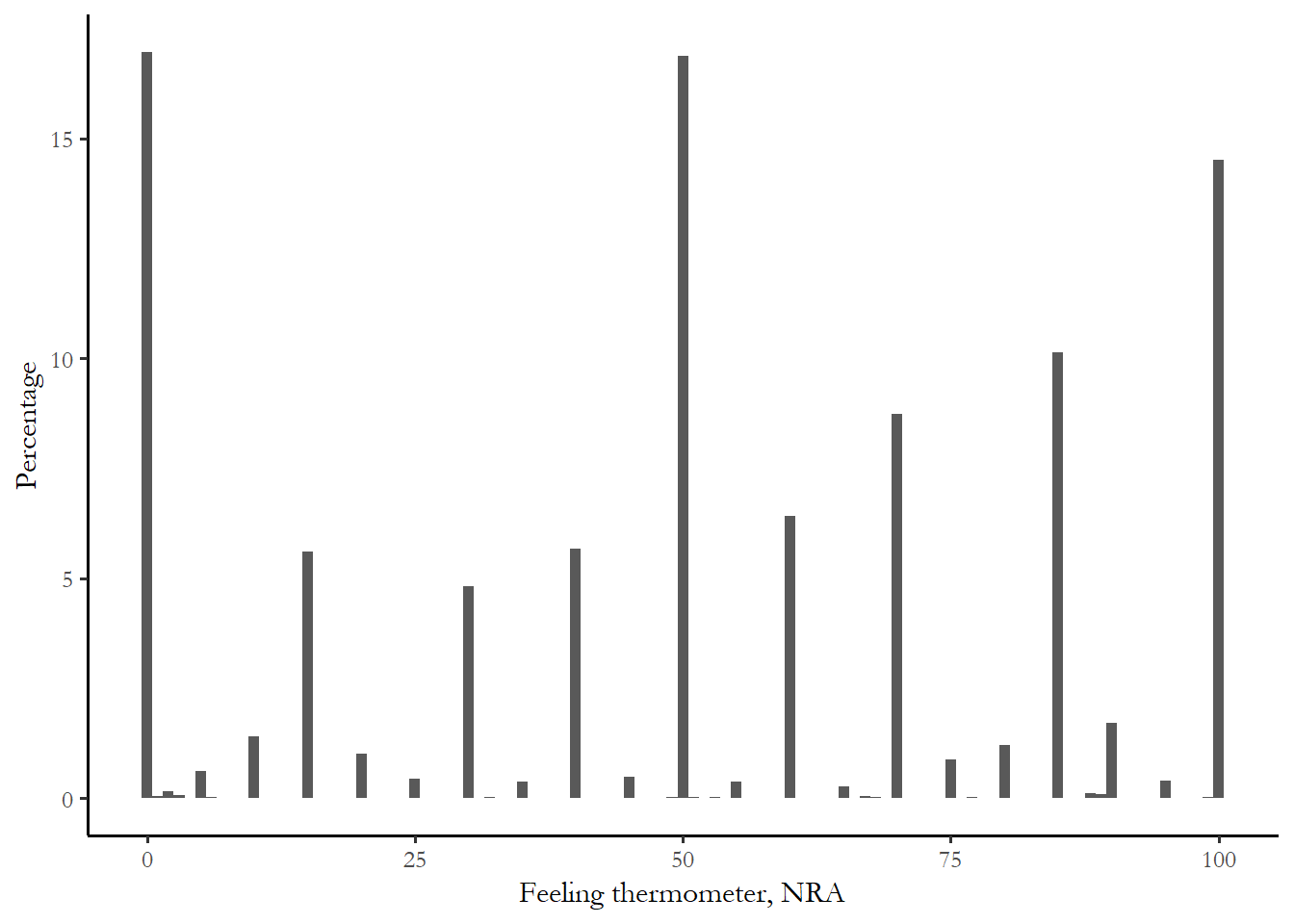
Table 4.2 Descriptive statistics. NRA feeling thermometer
| Descriptive statistics | |
|---|---|
| N | 2814 |
| Mean | 47.56 |
| Median | 50 |
| Variance | 977.56 |
| Standard deviation | 31.27 |
The 95% confidence interval in this case would be:
\[ 47.56 +/- (2 * 31.27 / \sqrt{2814}) = 47.56 +/- 0.59 \]
You don’t have to calculate this by hand - the information will be included in the output you use for the problem sets and papers. Again, this is precise - we know, with some certainty, that the population average is between 46.97 and 48.15.
We can replicate this calculation to compare smaller samples – men compared to women, white compared to minority. Instead of using the mean and standard error of the mean for the entire sample, we look at and compare two groups. If we can be 95% confident that the group means are different in the population, then we know we can safely make an inference about the population from our sample.
Gender and feelings toward the NRA
Will men and women have different attitudes toward the NRA? A lot of media coverage after the 2016 election focused on women’s activism and women’s voting, assuming or expecting that women would overwhelmingly support Democratic candidates, particular presidential nominee Hillary Clinton. Given that the Democratic party is more likely to advocate stronger restrictions on gun access, maybe women would dislike the NRA? We can test that expectation with a t-test. The results of this test are summarized in Table 4.3.
Table 4.3 Gender and the NRA feeling thermometer
Mean for Women = 45.69444
 Mean for Men = 49.46702
 t-test =  -3.054704
 p =  0.001
We only need to look at three numbers to understand this output – the average for men was 49.5 and the average for women was 45.7 – a small difference, but men slightly warmer. The significance level or p-value associated with this test is 0.000. What does this mean?
The actual value of the t-test is -3.05 and we use that number to come up with a significance level (also called a p-value). If there was no relationship between gender and the NRA thermometer (same exact means for men and women), the t-test would be 0.0 and the significance level would be 1.0. If the significance level is below 0.05, then we can be 95% confident that the groups are different in the population. In Table 4.1 the significance level (p) is less than 0.05, something less than 0.001.)
All statistics we use will be accompanied by a measure of significance – often denoted as “p” or the probability value. For our purposes, “p” is the probability that a test statistic of some value could be observed in a sample drawn from a population where the actual or true value of the test statistic is zero. There is a 0.00% probability that we could observe a t-test of -3.054 in the ANES if men and women had identical average NRA responses in the population
Note: this is very specific type of inference – we can learn something about the population from our small sample. If p < .05 then the observed difference between the two groups is statistically significant – this an arbitrary standard but a convention in social science. We will discuss this in a more systematic in the chapter on chi-square, but, for now, just remember the convention – p must be less than 0.05
This example also illustrates a key difference between “statistically significance” and “meaningful” - the difference between men and women is very small, a couple of points on the 100 point thermometer - so while we would observe a difference between men and women in the broader population, any differences would be very small.
Remember that we always report/discuss three things with a measure of association – size, direction, and significance. If a result is not significant, you can ignore size and direction – there is no effect, no link between \(X\) and \(Y\).
Race and feelings toward the NRA
Will white and minority respondents have different attitudes toward the NRA? The NRA is closely tied to the Republican Party, so might expect that this would translate into very different attitudes toward the NRA between whites and minorities. Results of a t-test are reproduced as Table 4.4.
Table 4.4 Race and the NRA
Mean for Minority (Black, Hispanic, or other) = 41.29045
 Mean for White = 50.94415
 t-test =  -7.788897
 p =  0.000
Again, three pieces of information tell the story. Race is a categorical or nominal variable with a couple of categories: 1. White, 2. Black, 3. Asian, 4. Native American, 5. Hispanic, 6. Other. The t-test permits us to compare White respondents (<2 on the scale) with all minorities (>=2). The average for white respondents was 50.9, but the average for minority respondents was 41.3 – much lower. The significance level in this case was again 0.000, much lower than 0.05. We can be confident that, in the larger population, white respondents have more favorable views of the NRA. Since the difference in means between White and Minority respondents is much larger than the difference between women and men, we know that race is a better predictor for understanding how someone feels about the NRA.
4.6 The t-test and Kalamazoo: a local connection
Student (Gossett) used several datasets from published work to demonstrate the usefulness of the t-test. One set of data was collected by a team of physicians at the Kalamazoo Psychiatric Hospital, comparing the effects of three different chemical compounds on patient sleep (published by A. R. Cushny and A. R. Peebles in the Journal of Physiology in 1906). Analyzing the data, Student demonstrated that small improved sleep times associated with one compound could just be due to chance, but larger improved sleep times associated with two of the other formulations indicated the treatments were effective. The research practices associated with the data collection and 1906 publication violate a number of standards that we regard as routine today - the original work was funded by the drug manufacturer (Merck), the patients did not consent to participating in the study, and there were no blinds - doctors knew who got which drugs. But the example has persisted in the statistical literature for 100 years. For details see Stigler (2019).
4.7 Conclusion
The t-test is a simple way to compare two groups and to verify that any differences between groups are not simply due to chance (sampling error). If we see a difference in sample means that is large enough to be statistically significant, we can be confident that repeated or larger samples would produce the same result.